Show equivalence of expressions for b

Return to Linear regression and correlation computing page
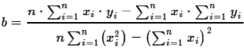
We have been given two ways to compute the value of the slope, b, in the linear regression equation y = a + b*x. Originally, for the paired sets of n values x_i and y_i we had

(1)

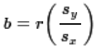
Then we were given

(2)

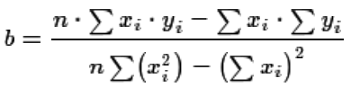
We want to show that these two, (1) and (2), are equivalent. First, let us agree that when we write the various summations we do not need to clutter the display with the i=1 below the Σ and the n above the Σ. Thus equation (1) is just restated as equation (3).

(3)

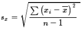
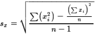
Then we recall that we define the standard deviation of a sample of x_i values as the root mean squared deviation from the mean, i.e., as shown in equation (4).

(4)

That equation, while absolutely correct and capturing the essence of the definition of s_x, is a bit hard to manipulate. When we first learned about the standard deviation of a sample we also learned that, with a bit of algebra, we could transform equation (4) into equation (5).

(5)

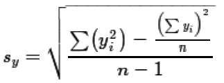
In a similar fashion we can write the standard deviation of the y_i values as equation (6).

(6)

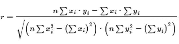
Then, we return to the equation for the correlation coefficient, r, given as equation (7).

(7)

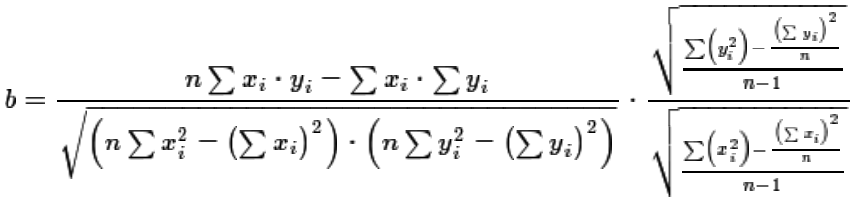
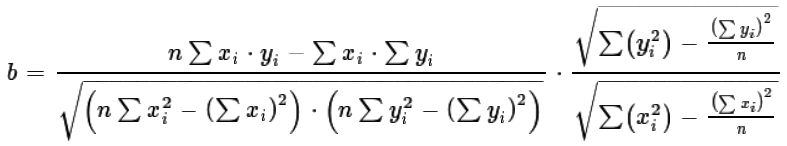
Using equations (7), (6), and (5) we can restate equation (2) as equation (8). Our goal is to rework equation (8) so that it looks just like equation (3), our original equation for the slope of a linear regression line.

(8)

Looking at the right end of equation (8) we see that both the square root in the numerator and the square root in the denominator have n - 1 in their respective denominators. These "cancel" each other and we can write equation (9) with a slightly simplified right end.

(9)

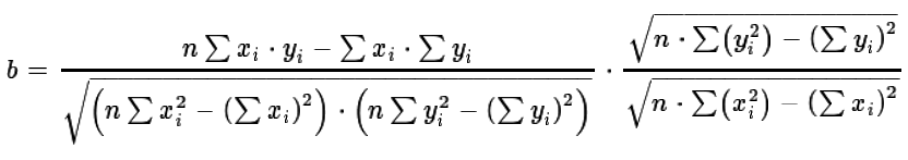
Again, looking at the square roots at the right end of equation (9), instead of have the difference of two terms the second of which is divided by n we can rewrite those roots as the quotient of the difference between n times the first summation minus the second summation and then divided by n. This is shown if equation (10).

(10)

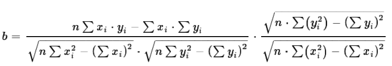
Equation (10) has the same characteristic at its right end as we saw back in equation (8), namely both roots at the right end have n in their respective denominator. Those values "cancel" to give us equation (11).

(11)

The denominator of the of the left factor of equation (11) has as its first factor the root of the product of two values. We can rewite that as the product of the root of the two values, yielding equation (12).

(12)

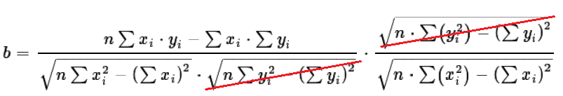
But, in equation (12) the second factor in denominator of the first fraction,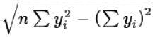

, is identical to the numerator of the second factor. These will "cancel" as shown in equation (13).

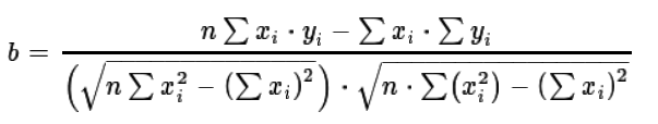
(13)

That leaves us with equation (14).

(14)

We observe that in equation (14) the denominator is just a square root times itself. We know that the square of the square root of a value is just that value. Thus we simplify equation (14) to be equation (15). But that is identical to equation (3), our original equation for the slope of the regression equation.

(15)